eRah Manual
v2.0.0
Xavier Domingo–Almenara
09 February, 2024
Source:vignettes/erah-manual.Rmd
erah-manual.RmdThis vignette presents eRah, an R package with an integrated design that allows for an innovative deconvolution of GC–MS chromatograms using multivariate techniques based on blind source separation (BSS), alignment of spectra across samples, and automatic identification of metabolites by spectral library matching. eRah outputs a table with compound names, matching scores and the area of the compound for each sample. eRah is designed in an open-structure, where researchers can integrate different algorithms for each step of the pipeline, i.e., compound deconvolution, alignment, identification or statistical analysis. eRah has been tested with GC-TOF/MS and GC-qTOF/MS (using nominal mass) equipment, and is compatible with different spectral databases.
Here, we integrate the downloadable version of the MassBank spectral library for an straightforward identification. If you use the package eRah in your analysis and publications please cite Domingo-Almenara et al. (2015) and Domingo-Almenara et al. (2016). Domingo-Almenara et al. (2016) is also referred for a more technical and detailed explanation about the eRah methods.
Installation
eRah can be installed from any CRAN repository, by:
install.packages('erah')Or from GitHub:
remotes::install_github('xdomingoal/erah-devel')Then loaded using:
##
##
##       _____        _
##      |  __ \      | |        eRah R package:
##   ___| |__) | __ _| |__       ----------------
##  / _ \  _   // _` |  _ \     Untargeted GC-MS metabolomics profiling
## |  __/ |  \ \ (_| | | | |
##  \___|_|   \_\__,_|_| |_|    Version 2.0.0
##
##  - Type 'citation('erah')' for citing this R package in publications.
##  - Type 'vignette('eRahManual', package='erah')' for a tutorial on eRah's usage.
##  - For bugs, problems and issues, please do not hesitate in contacting xavier.domingoa@eurecat.org or opening an issue on the Github repository (https://github.com/xdomingoal/erah-devel/issues).
Support
Any enquiries, bug reports or suggestions are welcome and they should be addressed to xavier.domingoa@eurecat.org. Alternatively, please file an issue (and, if possible, a reproducible example) at https://github.com/xdomingoal/erah-devel/issues.
##1. Introduction
eRah automatically detects and deconvolves the spectra of the compounds appearing in GC–MS chromatograms. eRah processes the raw data files (netCDF or mzXML) of a complete metabolomics experiment in an automated manner.
After that, compounds are aligned by spectral similarity and retention time distance. eRah computes the Euclidean distance between retention time distance and spectral similarity for all compounds in the chromatograms, resulting in compounds appearing across the maximum number of samples and with the least retention time and spectral distance.
Also, an (optional) missing compound recovery step, can be applied to recover those compounds that are missing in some samples. Missing compounds appear as a result of an incorrect deconvolution or alignment - due to a low compound concentration in a sample - , or because it is not present in the sample. This forces the final data table with compound names and compounds area, to not have any missing (zero) values.
Finally, identification of the found metabolites is conducted. A mean spectra from each group of aligned compounds is compared with a reference library. eRah includes a custom version of MassBank repository. Other libraries can imported with eRah (e.g., Golm Metabolome Database), and eRah’s deconvolved spectra can be exported for further comparison with NIST library.
##2. GC–MS Data Processing with eRah: a tutorial
In this section we show the processing of example samples from a spike-in experiment designed for interrogating data processing methods from the gcspikelite data package (Robinson 2018) that were analyzed using GC–MS. This sample set consists of nine samples with three triplicate classes.
The gcspikelite package can be installed from bioconductor using the BiocManager package:
install.packages('BiocManager')
BiocManager::install('gcspikelite')
The package and necessary data can be loaded using:
This tutorial shows how to deconvolve, align and identify the compounds contained in these samples. All the listed commands (script) to reproduce the following demo can by found by executing:
and then click on User guides, package vignettes and other documentation and on source from the ’eRah Manual’.
###2.1 Creating a new experiment
Prior to deconvolution, alignment and compound identification, we first need to setup a new experiment where the sample meta information is defined, such as file paths and class types. eRah provides two ways in which this can be achieved. The first of which requires only sample file paths and further sample class information is then added manually. The second derives sample class information and file paths from the underlying directory structure of a given experiment directory path.
####2.1.1 Using file paths only
Using this input method we first load the file paths of the given data set. For our example data set from the gcspikelite package we can do this by:
files <- list.files(system.file('data',package = 'gcspikelite'),full.names = TRUE)
files <- files[sapply(files,grepl,pattern = 'CDF')]
files then contains a vector of file paths to the nine
.CDF files needed for processing. An instrumental information table can
then be created from these using the following:
instrumental <- createInstrumentalTable(files)Further columns containing additional sample instrumental information can also be added to this table.
Next we can optionally define our class or phenotype information for our sample set. This can be done using the following, providing a vector of classes names that are associated with each file. Ensure that the order of the class affiliations match those of your file paths.
classes <- as.character(targets$Group[order(targets$FileName)])
phenotype <- createPhenoTable(files, cls = classes)
Similarly to the instrumental table, columns containing
additional sample instrumental information can also be added.
A new experiment can then be setup using our
instrumental and phenotype tables by:
ex <- newExp(instrumental = instrumental,
             phenotype = phenotype,
             info = "DEMO Experiment")
Where an experiment name can be defined using the info
argument. This creates a new MetaboSet object used for
storing the sample metadata and processing results.
####2.1.2 Using file directory structure
Alternatively, the structure of an experiment directory can be used to define the instrument and class information. The experiment directory should be organized as follows: all the samples related to each class have to be stored in the same folder (one folder = one class), and all the class-folders in one folder, which is the experiment folder (Figure 1). eRah also accepts only one class; in that case, only one class-folder has to be created inside an experiment-folder.
Figure 1 below shows the structure of an example experiment folder name PCOS. This contains two class-folders called ’CONTROL’ and ’DISEASE’, which each contain the sample files for that class. In this case these are the CON BASA 567795.mzXML, and CON BASA 574488.mzXML files in the CONTROL class.
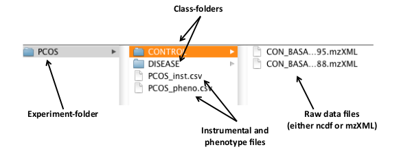
Figure 1: An example distribution of the raw data files and the class and experiment folders.
To create a new experiment we have to create first a .csv type file containing the name of the raw data files to process. The raw data files have to be in the same directory as the instrumental file. eRah also admits a phenotypic table which contains the classes of the samples. The instrumental data file is always needed but the phenotype file is optional. The instrumental table can have as many columns as desired, but it has to contain at least two columns named ’sampleID’ and ’filename’. The same is applicable to the phenotypic table, in this case the two necessary columns are ’sampleID’ and ’class’. Please note that capital letters of the column names must be respected and that ’sampleID’ is the column that relates the instrumental and phenotypic tables. These files can also be created automatically, execute the following command:
createdt('experiment_path/PCOS/')Where experiment_path is the path where the
experiment-folder is, and PCOS is the experiment-folder. Two things have
to be considered at this step: .csv files are different when created by
American and European computers, so errors may raise due to that fact.
Also, the folder containing the samples (in this case, the folder
’PCOS’, must contain only folders. If the folder ’PCOS’ contains files
(for example, already created .csv files), eRah will prompt an
error.
- Note that if you have an specific question about a function, you can
always access to the help of the function with a question mark before
the name of the function:
?createdt
The new experiment can then be created by loading the instrumental
and phenotypic tables into the workspace and supplying these to
newExp() as below:
instrumental <- read.csv('experiment_path/PCOS/PCOS_inst.csv')
phenotype <- read.csv('experiment_path/PCOS/PCOS_pheno.csv')

ex <- newExp(instrumental = instrumental,
             phenotype = phenotype,
             info = 'PCOS Experiment')
This creates a new MetaboSet object used for storing the
sample metadata and processing results.
####2.1.3 Accessing sample metadata
With metaData(), phenoData() and
expClasses() we can retrieve the instrumental data and the
experiment classes and the processing status:
metaData(ex)## # A tibble: 9 × 4
## sampleID filename date time
## <chr> <chr> <chr> <chr>
## 1 0709_468 /home/runner/work/_temp/Library/gcspikelite/data/0709_46… 2024… 08:4…
## 2 0709_470 /home/runner/work/_temp/Library/gcspikelite/data/0709_47… 2024… 08:4…
## 3 0709_471 /home/runner/work/_temp/Library/gcspikelite/data/0709_47… 2024… 08:4…
## 4 0709_474 /home/runner/work/_temp/Library/gcspikelite/data/0709_47… 2024… 08:4…
## 5 0709_475 /home/runner/work/_temp/Library/gcspikelite/data/0709_47… 2024… 08:4…
## 6 0709_479 /home/runner/work/_temp/Library/gcspikelite/data/0709_47… 2024… 08:4…
## 7 0709_485 /home/runner/work/_temp/Library/gcspikelite/data/0709_48… 2024… 08:4…
## 8 0709_493 /home/runner/work/_temp/Library/gcspikelite/data/0709_49… 2024… 08:4…
## 9 0709_496 /home/runner/work/_temp/Library/gcspikelite/data/0709_49… 2024… 08:4…
phenoData(ex)## # A tibble: 9 × 2
## sampleID class
## <chr> <chr>
## 1 0709_468 mmA
## 2 0709_470 mmD
## 3 0709_471 mmD
## 4 0709_474 mmA
## 5 0709_475 mmA
## 6 0709_479 mmD
## 7 0709_485 mmC
## 8 0709_493 mmC
## 9 0709_496 mmC
expClasses(ex)## Experiment containing 9 samples in 3 different type of classes named: mmA, mmC, mmD.
##
## Sample ID Class Type Processing Status
## 1 0709_468 mmA Not processed
## 2 0709_470 mmD Not processed
## 3 0709_471 mmD Not processed
## 4 0709_474 mmA Not processed
## 5 0709_475 mmA Not processed
## 6 0709_479 mmD Not processed
## 7 0709_485 mmC Not processed
## 8 0709_493 mmC Not processed
## 9 0709_496 mmC Not processed###2.2 Compound deconvolution
The compounds in data are deconvolved using
deconvolveComp(). This function requires a
Deconvolution parameters object, that can be created with
setDecPar function, containing the parameters of the
algorithm as shown as follows:
The peak width value (in seconds) is a critical parameter that conditions the efficiency of eRah, and also the masses to exclude have an important role in GC–MS-based metabolomics experiments.
Peak width parameter: typically, this value should be the less than half of the mean compound width. For this experiment, the average peak width is between 2 and 2.5 seconds, so we selected 1 second peak width. The lower this parameter is set to, the more sensibility to deconvolve co-eluted compounds, but it also may increase the number of false positive compounds. If is set too low the algorithm will generate too false positives compounds, which this usually means that one single compound will be detected twice. If the parameter value is increased, the algorithm may fail in separate co-eluted compounds, leading to generate less false positives but loosing capacity of detection.
Masses to exclude: masses m/z 73, 74, 75, 147, 148, 149 are recommended to be excluded in the processing and subsequent steps, since these are ubiquitous mass fragments typically generated from compounds carrying a trimethylsilyl moiety. If the samples have been derivatized, including these masses will only hamper the deconvolution process; this is because an important number of compounds will share these masses leading to a poorer selectivity between compounds. Also, in complex GC–MS-based metabolomics samples, we also recommend excluding all masses from 1 to 69 Da, for the same reasons. Those masses are generated from compounds with groups that are very common for a large number of compounds in metabolomics, leading to a poorer selectivity between compounds. Although those masses are also the most intense m/z in the compounds spectra, eRah will automatically set the used library’s masses to zero, so it does not affect spectral matching and identification.
eRah also supports parallel processing at this step using the future package. This enables the faster processing of large sample sets.
By default, deconvolution will be done on each file sequentially.
However, parallel processing can be activated prior to to this by
specifying a parallel backend using plan(). The following
example specifies using the multisession backend (muliple
background R sessions) with two worker processes.
plan(future::multisession,workers = 2)See the future package documentation for more information on the types of parallel backends that are available.
The samples can then be deconvolved using:
ex <- deconvolveComp(ex, ex.dec.par)##
## Deconvolving compounds from /home/runner/work/_temp/Library/gcspikelite/data/0709_468.CDF ... Processing 1 / 9##
## Deconvolving compounds from /home/runner/work/_temp/Library/gcspikelite/data/0709_470.CDF ... Processing 2 / 9##
## Deconvolving compounds from /home/runner/work/_temp/Library/gcspikelite/data/0709_471.CDF ... Processing 3 / 9##
## Deconvolving compounds from /home/runner/work/_temp/Library/gcspikelite/data/0709_474.CDF ... Processing 4 / 9##
## Deconvolving compounds from /home/runner/work/_temp/Library/gcspikelite/data/0709_475.CDF ... Processing 5 / 9##
## Deconvolving compounds from /home/runner/work/_temp/Library/gcspikelite/data/0709_479.CDF ... Processing 6 / 9##
## Deconvolving compounds from /home/runner/work/_temp/Library/gcspikelite/data/0709_485.CDF ... Processing 7 / 9##
## Deconvolving compounds from /home/runner/work/_temp/Library/gcspikelite/data/0709_493.CDF ... Processing 8 / 9##
## Deconvolving compounds from /home/runner/work/_temp/Library/gcspikelite/data/0709_496.CDF ... Processing 9 / 9## Compounds deconvolved
ex## A "MetaboSet" object containing 9 samples
##
## Data processed with
## Info attached to this experiment:
## DEMO ExperimentData can be saved and loaded at any stage of the process by:
###2.3 Alignment
Alignment is executed with alignComp(). The parameters
also have to be set prior to this.
ex.al.par <- setAlPar(min.spectra.cor = 0.90, max.time.dist = 3, mz.range = 70:600)The parameters are min.spectra.cor,
max.time.dist and mz.range. The
min.spectra.cor (Minimum spectral correlation) value - from
0 (non similar) to 1 (very similar) - sets how similar two or more
compounds have be to be considered for alignment between them. We can be
restrictive with this parameter, as if one compound is not detected in
some samples, we can retrieve it later by the ’missing compound
recovery’ step. Also, we impose a maximum disalignment distance of 3
seconds (max.time.dist). This value (in seconds) sets how
far two or more compounds can be considered for alignment between them.
mz.range is the range of masses that is considered when
comparing spectra. We set that only the masses from 70 to 600 are taken
into account, for the reasons commented above in the ’Masses to exclude’
point.
Alignment can be performed by:
ex <- alignComp(ex, alParameters = ex.al.par)

ex
## A "MetaboSet" object containing 9 samples
##
## Data processed with
## Info attached to this experiment:
## DEMO Experiment-
Aligning large ammout of samples: For experiments
containing more than 100 (Windows) or 1000 (Mac or Linux) samples,
alignment could lead to errors or show a poor run-time performance. In
those cases alignment can be conducted by block segmentation. For more
details about
alignComp()access help using?alignComp
We can decide to execute the missing compound recovery step (and
retrieve the compounds that have missing values - have not been found -
in certain samples) or also identify the compounds without applying
recMissComp(). In other words, the missing compound
recovery step is optional. Here, we apply the missing recovery step to
later identify the compounds.
###2.4 Missing compound recovery
The missing compound recovery step only requires to indicate the
number of minimum values for which a compound wants to be ’re-searched’
in the samples. If a compound appears in at least the same or more
samples than the minimum samples value (min.samples), then,
this compound is searched in the rest of the samples where its
concentration has not been registered. To do so:
ex <- recMissComp(ex, min.samples = 6)##
## Updating alignment table...
## Model fitted!
ex## A "MetaboSet" object containing 9 samples
##
## Data processed with
## Info attached to this experiment:
## DEMO Experiment-
Missing compound recovery: The min.samples
parameter sets the number of samples from the total number of samples.
Also, this parameter should be large, in alignment with the dimension of
the number of samples in the experiment. If set too low, a higher number
of false positives are expected. A recommended strategy is to first
evaluate the average number of samples where the compounds appear, by
executeing
alignList ()oridList()- after being identified - functions (explained in the following sections). Warning: if we have already identified the compounds, we always have to re-identify the compounds after executing the missing compound recovery step, byidentifyComp(), as explained in the following sections.
###2.5 Identification
The final processing step is to identify the previously aligned compounds and assign them a putative name. eRah compares all the spectra found against a reference database. This package includes a custom version of the MassBank MS library, which is selected as default database for all the functions. However, we strongly encourage the use of the Golm Metabolome Database (GMD). GMD importation is described in following sections.
Identification can be executed by identifyComp, and accessed by idList as follows:
ex <- identifyComp(ex)## Constructing matrix database...
## Comparing spectra...
## Done!## # A tibble: 8 × 4
## AlignID tmean FoundIn Name.1
## <dbl> <dbl> <dbl> <chr>
## 1 13 5.79 9 Harmaline (1TMS)
## 2 17 5.88 9 2-Hydroxypyridine
## 3 16 5.96 9 2-Hydroxypyridine
## 4 25 6.08 9 2'-Deoxyadenosine (3TMS)
## 5 27 6.18 9 2,3-Bisphospho-glycerate
## 6 35 6.36 9 DL-2,3-Diaminopropionic acid (2TMS)
## 7 39 6.50 9 (R)-(-)-Phenylephrine (2TMS)
## 8 44 6.63 9 Malonic acid (2TMS)###2.6 Results and visualization
The identification list can be obtained using:
idList(ex)## # A tibble: 124 × 18
## AlignID tmean FoundIn Name.1 MatchFactor.1 DB.Id.1 CAS.1 Formula.1 Name.2
## <dbl> <dbl> <dbl> <chr> <chr> <chr> <chr> <chr> <chr>
## 1 13 5.79 9 Harmaline… 88.58 "434" 6027… "C16H22N… Dopam…
## 2 17 5.88 9 2-Hydroxy… 87.89 " 25" 142-… "" 4-Hyd…
## 3 16 5.96 9 2-Hydroxy… 99.27 " 25" 142-… "" 4-Hyd…
## 4 25 6.08 9 2'-Deoxya… 59.47 "372" 1637… "C22H45N… 2'-De…
## 5 27 6.18 9 2,3-Bisph… 75.78 "456" 1443… "" DL-Ho…
## 6 35 6.36 9 DL-2,3-Di… 94.62 "334" 5487… "C18H48N… Oxami…
## 7 39 6.50 9 (R)-(-)-P… 94.10 "322" 61-7… "C18H37N… (-)-E…
## 8 44 6.63 9 Malonic a… 52.87 "252" 141-… "C13H28O… Dihyd…
## 9 45 6.66 9 L-Alanine… 99.11 "335" 56-4… "C12H31N… (R)-(…
## 10 51 6.75 9 L-Alanine… 99.15 "335" 56-4… "C12H31N… (R)-(…
## # ℹ 114 more rows
## # ℹ 9 more variables: MatchFactor.2 <chr>, DB.Id.2 <chr>, CAS.2 <chr>,
## # Formula.2 <chr>, Name.3 <chr>, MatchFactor.3 <chr>, DB.Id.3 <chr>,
## # CAS.3 <chr>, Formula.3 <chr>The alignment list can be returned using:
alignList(ex)## # A tibble: 124 × 13
## AlignID Factor tmean FoundIn `0709_468` `0709_470` `0709_471` `0709_474`
## <int> <chr> <dbl> <dbl> <dbl> <dbl> <dbl> <dbl>
## 1 13 Factor #13 5.79 9 46805 43277 49578 40353
## 2 17 Factor #17 5.88 9 153248. 197488. 102053 105891
## 3 16 Factor #16 5.96 9 427706 533857 525813 588514
## 4 25 Factor #25 6.08 9 69133 94935 93110 90711
## 5 27 Factor #27 6.18 9 406890 624249. 484318 456469
## 6 35 Factor #35 6.36 9 33943 47453 44354 34835
## 7 39 Factor #39 6.50 9 26594 35572 37724 29419
## 8 44 Factor #44 6.63 9 4549988 4743601 4642613 5242164
## 9 45 Factor #45 6.66 9 3022490 1620110 1544762 1223930
## 10 51 Factor #51 6.75 9 818746 942865 923088 811215
## # ℹ 114 more rows
## # ℹ 5 more variables: `0709_475` <dbl>, `0709_479` <dbl>, `0709_485` <dbl>,
## # `0709_493` <dbl>, `0709_496` <dbl>And the final data list can be returned using:
dataList(ex)## # A tibble: 124 × 27
## AlignID tmean FoundIn Name.1 MatchFactor.1 DB.Id.1 CAS.1 Formula.1 Name.2
## <dbl> <dbl> <dbl> <chr> <chr> <chr> <chr> <chr> <chr>
## 1 13 5.79 9 Harmaline… 88.58 "434" 6027… "C16H22N… Dopam…
## 2 16 5.96 9 2-Hydroxy… 99.27 " 25" 142-… "" 4-Hyd…
## 3 17 5.88 9 2-Hydroxy… 87.89 " 25" 142-… "" 4-Hyd…
## 4 25 6.08 9 2'-Deoxya… 59.47 "372" 1637… "C22H45N… 2'-De…
## 5 27 6.18 9 2,3-Bisph… 75.78 "456" 1443… "" DL-Ho…
## 6 35 6.36 9 DL-2,3-Di… 94.62 "334" 5487… "C18H48N… Oxami…
## 7 39 6.50 9 (R)-(-)-P… 94.10 "322" 61-7… "C18H37N… (-)-E…
## 8 44 6.63 9 Malonic a… 52.87 "252" 141-… "C13H28O… Dihyd…
## 9 45 6.66 9 L-Alanine… 99.11 "335" 56-4… "C12H31N… (R)-(…
## 10 51 6.75 9 L-Alanine… 99.15 "335" 56-4… "C12H31N… (R)-(…
## # ℹ 114 more rows
## # ℹ 18 more variables: MatchFactor.2 <chr>, DB.Id.2 <chr>, CAS.2 <chr>,
## # Formula.2 <chr>, Name.3 <chr>, MatchFactor.3 <chr>, DB.Id.3 <chr>,
## # CAS.3 <chr>, Formula.3 <chr>, `0709_468` <dbl>, `0709_470` <dbl>,
## # `0709_471` <dbl>, `0709_474` <dbl>, `0709_475` <dbl>, `0709_479` <dbl>,
## # `0709_485` <dbl>, `0709_493` <dbl>, `0709_496` <dbl>From the table returned by idList(ex), we see that
gallic acid is appearing at minute 7.81 with an AlignID number #84. Let
us have a look to its profile with the function plotProfile:
- Execute
?alignList, to access to the help of alignList function with a detailed explanation of each column in an align list.
plotProfile(ex, 84)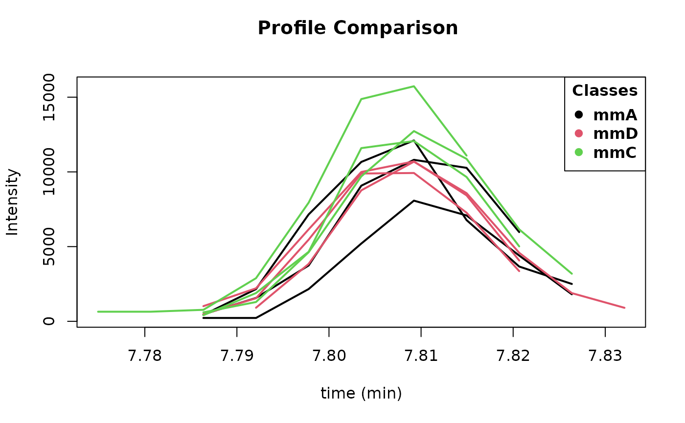
Figure 2: Image from plotProfile(ex,84).
This displays Figure 2. Its spectra can be also be plotted and compared with the reference spectra using the function plotSprectra, which displays Figure 3:
plotSpectra(ex, 84)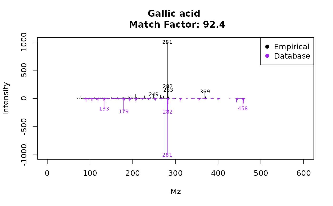
Figure 3: Image from plotSpectra(ex,84).
The plotSpectra function has a lot of possibilities for plotting, to
know more access to its particular help by executing
?plotSpectra. For example, eRah allows a rapid assessment
for visualizing the second hit returned in the case of compound align ID
#41 (Urea). To do so:
plotSpectra(ex, 84, 2, draw.color = "orange")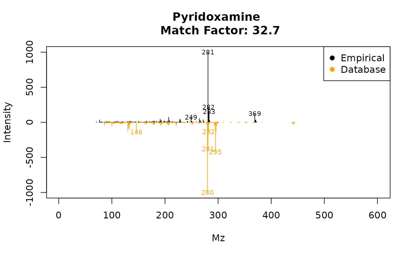
Figure 4: Image from
plotSpectra(ex,84, 2, draw.color=’orange3’).
This plots Figure 4, which is a comparison of the empirical spectrum found, with the second most similar metabolite from the database (in this case pyridoxamine). From the figure, it is clear that eRah returned the first hit correctly, as this spectra is more similar to gallic acid than to pyridoxamine.
##3. Importing and customizing mass spectral libraries
###3.1 Using the Golm Metabolome Database
Users may import their own mass spectral libraries. We strongly
recommend using the Golm Metabolome Database (GMD) with eRah. To use the
GMD, first, we have to download it from its webpage, by
downloading the file ”GMD 20111121 VAR5 ALK MSP.txt” or ”GMD 20111121
MDN35 ALK MSP.txt”, depending on which type of chromatographic columns
(VAR5 or MDN35) are we using. If you are not interested in using any
retention index information, then both files can be used indistinctly.
Then, we can load the library with the function
importMSP():
g.info <- "
GOLM Metabolome Database
------------------------
Kopka, J., Schauer, N., Krueger, S., Birkemeyer, C., Usadel, B., Bergmuller, E., Dor-
mann, P., Weckwerth, W., Gibon, Y., Stitt, M., Willmitzer, L., Fernie, A.R. and Stein-
hauser, D. (2005) GMD.CSB.DB: the Golm Metabolome Database, Bioinformatics, 21, 1635-
1638."

golm.database <- importGMD(filename="GMD_20111121_VAR5_ALK_MSP.txt",
                           DB.name="GMD",
                           DB.version="GMD_20111121",
                           DB.info= g.info,type="VAR5.ALK")

# The library in R format can now be stored for a posterior faster loading
save(golm.database, file= "golmdatabase.rda")
We can substitute the default eRah database object
mslib, for our custom database, by the following code:
load("golmdatabase.rda")
mslib <- golm.database
This allows executing all the functions without the need of always
setting the library parameter. If we do not replace the
mslib object as shown before, we have to use the new
library (in this case golm.database) in all the functions,
for example:
findComp(name = "phenol", id.database = golm.database)###3.2 Using in-house libraries
Other MSP-formatted libraries can be also imported. The procedure is
the same as for the GMD database, with the only exception is that the
function is importMSP instead of importGMD.
Access to specific importMSP help in R
(?importMSP) for details on database MSP input format.
##4 Exporting spectra: comparison with NIST
Users may export their results to MSP format or CEF format for
comparison with NIST MS Search software (MSP), or to compare spectra
with NIST through the MassHunter workstation (CEF). Users are referred
to exportMSP and exportCEF functions help for
more details.
##5. Final Summary To complement the given tutorial, the user may access to the particular help for each function, as shown before. Also, and for more details, please read the original article. Here, we show a figure (Figure 5) with all the available functions.
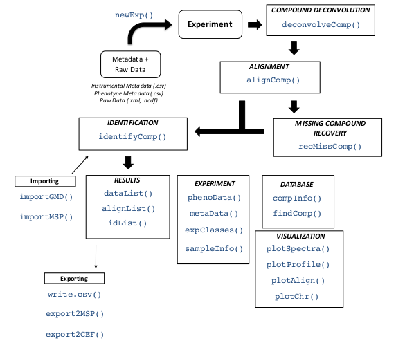
Figure 5: eRah summary of functions.
##6. References